
.png&blockId=21b2dc3e-f514-818b-b72b-f9aade6351bf)

Task : 메인 가설
리뷰 수, 최근 리뷰 존재, 매출 추정치가 포함→ 인기 점수
메인 가설
"도심 지역에서 'Entire home/apt'(아파트형) 숙소는 다른 방 타입에 비해 인기가 많을 것이다.
→ 가설 설정 이유 : 도심지역에 'Entire home/apt'(아파트형) 숙소가 가장 많이 있기 때문이다.
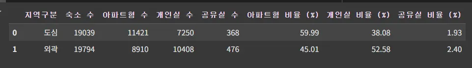
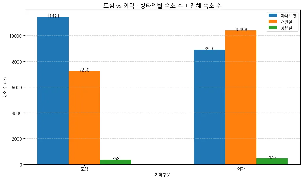
도심 vs 외곽 숙소 수 비교 및 방타입 별 수 비교
# 방타입별 숙소 수 계산
pivot = df_filtered.pivot_table(index='city_and_suburb',
columns='room_type',
aggfunc='size',
fill_value=0).reset_index()
# 전체 숙소 수도 함께 계산
pivot['숙소 수'] = pivot[['Entire home/apt', 'Private room', 'Shared room']].sum(axis=1)
# 각 방타입 비율 계산
pivot['아파트형 비율 (%)'] = (pivot['Entire home/apt'] / pivot['숙소 수'] * 100).round(2)
pivot['개인실 비율 (%)'] = (pivot['Private room'] / pivot['숙소 수'] * 100).round(2)
pivot['공유실 비율 (%)'] = (pivot['Shared room'] / pivot['숙소 수'] * 100).round(2)
# 열 순서 재정렬
pivot = pivot[['city_and_suburb', '숙소 수', 'Entire home/apt', 'Private room', 'Shared room',
'아파트형 비율 (%)', '개인실 비율 (%)', '공유실 비율 (%)']]
# 컬럼명 한글로 변경
pivot.columns = ['지역구분', '숙소 수', '아파트형 수', '개인실 수', '공유실 수',
'아파트형 비율 (%)', '개인실 비율 (%)', '공유실 비율 (%)']
# 출력
pivot
Python
복사
주요 인사이트
•
외곽 지역의 숙소 수가 약간 더 많음.
•
도심에서는 'Entire home/apt'(아파트형) 숙소 비율이 가장 높음 (59.99%).
•
반면 외곽은 개인실(Private room) 비율이 가장 높음 (52.58%).
Task : "도심 지역에서 'Entire home/apt'(아파트형) 숙소는 다른 방 타입에 비해 인기도 점수가 더 높을 것이다. ⇒ 증명 시작
0.
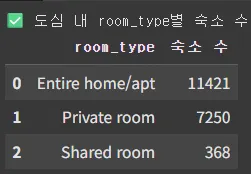
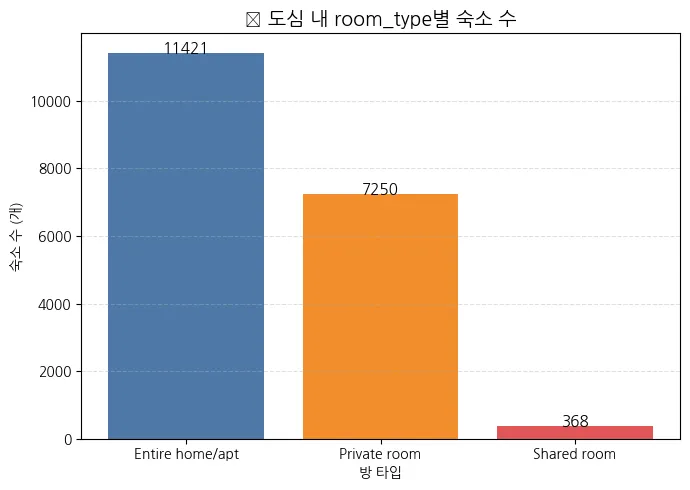
도심 내 room_type별 숙소 수 다시 확인.
# 도심 지역에서 room_type별 숙소 수 집계
city_room_counts = df_filtered[df_filtered['city_and_suburb'] == '도심']['room_type'].value_counts().reset_index()
city_room_counts.columns = ['room_type', '숙소 수']
# 정렬해서 보기 좋게
city_room_counts = city_room_counts.sort_values(by='숙소 수', ascending=False).reset_index(drop=True)
# 출력
print("✅ 도심 내 room_type별 숙소 수:")
display(city_room_counts)
Python
복사
1.
도심 방 타입 별 popularity_score 평균 구하기
# 도심 지역만 필터링
df_downtown = df_filtered[df_filtered['city_and_suburb'] == '도심']
# 방타입별 popularity_score 평균 계산
avg_score_by_room = df_downtown.groupby('room_type')['popularity_score'].mean().reset_index()
# 점수 내림차순 정렬
avg_score_by_room = avg_score_by_room.sort_values(by='popularity_score', ascending=False)
# 확인
# 소수점 2자리 반올림 후 출력
display(avg_score_by_room.round(2))
Python
복사
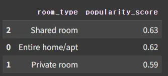
요약 및 결론
•
공유형(Shared room)
→ 평균 인기 점수는 가장 높음 (0.63)
→ 단, 숙소 수가 너무 적어 일반화에는 어려움
→ 운영 효율은 높을 수 있으나, 확장성·시장성은 낮음
•
아파트형(Entire home/apt)
→ 평균 인기 점수 0.62로 매우 높음
→ 도심 내 가장 많은 수의 숙소를 차지
→ 안정적이며 실질적인 인기 숙소 유형
•
개인실(Private room)
→ 평균 인기 점수 0.59
→ 상대적으로 낮지만, 여전히 수요 존재
→ 1인 여행객이나 가족 단위 이용 가능성 해석
결과
“단순 평균 기준 Shared room이 가장 높은 점수를 보였으나, 전체 숙소 수가 적어 일반화에는 무리가 있으며, 실제 시장 영향력은 Entire home/apt가 더 크다.”
이 상태에서 단순 평균만 보면 왜곡 됨.
이 상태에서 단순 평균만 보면 왜곡 됨. 가중 평균 사용하기 ⇒ 표본 차이 때문!!!
가중 평균 인기점수( 도심 방타입 별)
import pandas as pd
# 데이터 예시 (이미 유진님이 갖고 있는 걸 기반으로 재구성)
data = {
'room_type': ['Entire home/apt', 'Private room', 'Shared room'],
'count': [11421, 7250, 368],
'popularity_score': [0.62, 0.59, 0.63]
}
df_score = pd.DataFrame(data)
# 전체 숙소 수
total_count = df_score['count'].sum()
# 가중 평균 기여도 컬럼 추가
df_score['weighted_contribution'] = (df_score['popularity_score'] * df_score['count']) / total_count
# 가중 평균 점수
weighted_avg_score = df_score['weighted_contribution'].sum()
# 출력
print("가중 평균 인기점수 (도심 전체 기준):", round(weighted_avg_score, 3))
display(df_score.round(3))
Python
복사
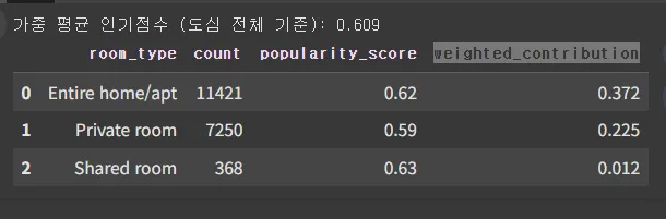
⇒ 가중 평균 기준으로 봤을 때,
가설: "도심 지역에서 'Entire home/apt'(아파트형) 숙소는 다른 방타입에 비해 인기도 점수가 더 높을 것이다."
가 참이다.!!!!
가설 정리 및 결론 제안
가설: "도심 지역에서 'Entire home/apt'(아파트형) 숙소는 다른 방타입에 비해 인기도 점수가 더 높을 것이다."
참!!!!
즉, "도심 지역에서 'Entire home/apt'(아파트형) 숙소는 다른 방타입에 비해 인기도 점수가 더 높다!!
세부 분석
세부 분석
"도심 지역 내 'Entire home/apt'(아파트형) 숙소 중 상위 25%와 하위 25%의 차이 분석
1.
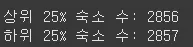
도심 지역 내 'Entire home/apt'(아파트형) 숙소 중 상위 25%와 하위 25% 수 비교
# 1. 분석 대상 필터링
target = df_filtered[
(df_filtered['city_and_suburb'] == '도심') &
(df_filtered['room_type'] == 'Entire home/apt')
]
# 2. 해당 popularity_score 기준 25% 분위값 계산
q1 = target['popularity_score_도심_Entire_home/apt'].quantile(0.25)
q3 = target['popularity_score_도심_Entire_home/apt'].quantile(0.75)
# 3. 상위 / 하위 25% 필터링
bottom_25 = target[target['popularity_score_도심_Entire_home/apt'] <= q1]
top_25 = target[target['popularity_score_도심_Entire_home/apt'] >= q3]
# 4. 숙소 수 확인
print("상위 25% 숙소 수:", len(top_25))
print("하위 25% 숙소 수:", len(bottom_25))
Python
복사
2. 도심 아파트형태 숙소 상위,하위 25% 의 예약가능일수 확인
# 필터링
target = df_filtered[
(df_filtered['city_and_suburb'] == '도심') &
(df_filtered['room_type'] == 'Entire home/apt')
].copy()
# 분위수 계산 (슬래시 컬럼은 .loc로 안정 접근)
score_col = "popularity_score_도심_Entire_home/apt"
q1 = target.loc[:, score_col].quantile(0.25)
q3 = target.loc[:, score_col].quantile(0.75)
# 상/하위 25%
top_25 = target[target[score_col] >= q3].copy()
bottom_25 = target[target[score_col] <= q1].copy()
# 구간화 함수
def classify_avail_days(days):
if days == 0:
return "0일"
elif days <= 90:
return "1~90일"
elif days <= 180:
return "91~180일"
elif days <= 270:
return "181~270일"
elif days < 365:
return "271~364일"
else:
return "365일"
# 구간 추가
top_25['availability_range'] = top_25['availability_365'].apply(classify_avail_days)
bottom_25['availability_range'] = bottom_25['availability_365'].apply(classify_avail_days)
# 구간 순서 정의
ordered_ranges = ["0일", "1~90일", "91~180일", "181~270일", "271~364일", "365일"]
# 결과표 구성
final_result_df = pd.DataFrame({
"상위 25%": [top_25['availability_range'].value_counts().get(r, 0) for r in ordered_ranges],
"하위 25%": [bottom_25['availability_range'].value_counts().get(r, 0) for r in ordered_ranges]
}, index=ordered_ranges)
# 보기 좋게 출력
display(final_result_df)
Python
복사
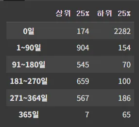
총 11421개 중
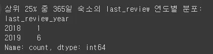
⇒ 라스트 리뷰가 2018인건 봐야 하는건 맞는데 , 데이터가 날라가는 것이 문제다.
상위 25% 중 availability_365 == 0 인 숙소들의 평균 리뷰 수
# 상위 25% 중 availability_365 == 0 인 숙소들의 평균 리뷰 수
top_25[top_25['availability_365'] == 0]['number_of_reviews'].describe()
Python
복사
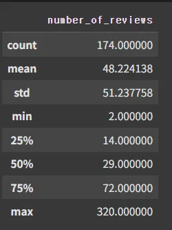
인기가 많아서 꽉 찼다고 설명 가능
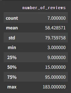
상위 25% 중 availability_365 == 365 인 숙소들의 평균 리뷰 수
# 상위 25% 중 availability_365 == 0 인 숙소들의 평균 리뷰 수
top_25[top_25['availability_365'] == 365]['number_of_reviews'].describe()
Python
복사
상위 25% 중 [availability_365 == 365] 인 숙소의 last_review 연도별 분포
# 1️⃣ 도심 아파트형 필터링
target = df_filtered[
(df_filtered['city_and_suburb'] == '도심') &
(df_filtered['room_type'] == 'Entire home/apt')
].copy()
# 2️⃣ 상위 25% 필터링
q3 = target['popularity_score_도심_Entire_home/apt'].quantile(0.75)
top_25 = target[target['popularity_score_도심_Entire_home/apt'] >= q3].copy()
# 3️⃣ availability_365 == 365인 숙소 필터링
top_25_365 = top_25[top_25['availability_365'] == 365].copy()
# 4️⃣ last_review 연도 추출 및 분포 확인
top_25_365['last_review_year'] = pd.to_datetime(top_25_365['last_review'], errors='coerce').dt.year
review_year_dist_top = top_25_365['last_review_year'].value_counts().sort_index()
# 5️⃣ 결과 출력
print("상위 25% 중 365일 숙소의 last_review 연도별 분포:")
print(review_year_dist_top)
Python
복사
내가 세운 운영 중 비운영 기준
왜 지금 운영과 비 운영을 나눠?
상위 25% vs 하위 25% 비교
하위 25% 지역 분포 확인 TOP 10
상위 25% 지역 분포 확인 TOP 10
여기까지 인사이트 도출
상위 25% 하위25% 숙소 가격 분포 확인
운영 특성을 단어를 나눠서. 비교 분석함.
- 운영 방식( 가격대, 지역별, 최소 숙박일 수 )
- 가격대가 다를 것이다. 하나하나를 가설로 만들어버리자.
통계
상위 25% 에서 가격대는 인기도에 영향을 미칠까? 통계 분석